Approximating the Yardage Value of a Pass Deflection in the Aggregate

Rich Sherman administers a critical pass deflection.

As adumbrated in the previous post, I wanted to quantify the yardage value of a pass deflection (PD). I will wait to consider the effect of team defense and special teams in a future post. I apologize to readers anxiously awaiting that analysis.

A PD occurs when a defender deflects a pass or dislodges a to-be-caught ball from the grasp of a receiver or otherwise actively prevents a reception (without penalty). A PD is a productive play for the defense and an unproductive play for the offense. There is a caveat to that, however: a PD on 1st, 2nd, or 3rd down is diminutively productive for the offense in that it ensures another down (i.e., no turnover).

There is no progress in obtaining a 1st down on the down in which a PD occurs. Likewise, a PD reduces by 1 the quantity of downs available to the offense. Ultimately, a PD indefinitely results in zero yards gained offensively or allowed defensively. Because of this, established per-pass or -attempt values such as Y/C-, Y/A- or N/YA-allowed would be inaccurate because those values are calculated using yardage of offensively productive passes (i.e., yardage incurred on plays generating 1st downs and TDs).

Concretely, a down of zero gain yields a yardage value of zero, duh. Abstractly, the yardage value of a down with zero gain—and thus, the yardage value of a PD—varies depending upon context, of course. Game importance, game score, down, and the yards needed to secure another 1st down are each salient.  So, for me, the dilemma entailed identifying a team-specific, discrete yardage value that, in the aggregate, accurately represents a PD.

Additional complexities arise because a PD is but one of many unproductive—or less than optimally productive—offensive passing outcomes. First quarter, tie game, 3rd and 10 at their own 20, for example, the QB hits his targeted WR on a bubble. As the WR secures the ball he is tackled harmlessly for a gain of zero. The play was unproductive because the team fails to secure a 1st down. Consider the same 3rd and 10 but instead, the QB successfully passes to the WR for a gain of 8. The offense fails to secure a 1st down and punts away possession. Although this second example is also unproductive, it is marginally more productive than the first example-play because the 8-yard gain conceivably reduces the opponent’s starting position. Thus, we need to quantify unproductiveness.

Metrics judiciously more refined and discriminative than anything you’ll probably ever read about on POTH provide some insight. For instance, Football Outsiders have identified expectations of offensive success. An offense shall accrue 45%, 60%, or 100% of needed yards on 1st, 2nd, or 3rd down, respectively. On 1st and 10, then, an offense ought to gain at least 4.5 yards  for a play to be considered productive; for 2nd and X, 60% of X; and for 3rd and X, at least X yards. With this model then, offensive unproductiveness is the failure to obtain those thresholds and the PD-yards value should, given my definition, be equivalent to the average yards allowed on unproductive pass plays. Readily obtainable via the publicly available play-by-play data (here and here) are the yards generated on unproductive completions.

To review, we are obtaining 6 summative data points per team per season: 

• quantity of completions of <50% yards to go on 1st down and the
• quantity of yards accumulated therein; 
• completions of <60% yards to go on 2nd down and the 
• accumulated yards; and
• completions of <X yards to go on 3rd and X and the
• yards on 3rd and X.

I’d like to add that I considered using the difference of unproductive yards and yards to go as a measure in the computation of PD yards. My suspicion was that that difference would yield larger values for defenses that limited offensive opponents' progress and forced longer ‘yards to go’ situations, thus larger values would reflect better defensive play. However, I decided against this because cursory analysis disconfirmed my suspicions.

Table 1. Descriptive statistics for average yards allowed per unproductive completion by team defenses, 2010-2014.

I obtained the data points described above for all NFL teams in the 2010 through 2014 regular seasons. Table 1 contains some descriptive stats for the average yards allowed per unproductive completion per team defense. Across seasons, the 2013 Buffalo Bills were lowest and the 2011 NY were highest. Across all seasons, there is slightly significant kurtosis and minute skewness but, with the exception of 2013, each individual season is normally distributed. Additional statistical procedures reveal that the effect of PD yards on starting position is almost entirely attributable to the action of PDs and not unproductive yardage.¹

I could discuss the weaknesses of this approach of quantifying PD yards but I really don’t feel like it. Instead, I provide an anecdote in the following paragraph providing some perspective on the notion of productivity. Likewise, I provide a table at the close of the post which displays the simple correlations of PD yards. Aside from developing a method of quantifying PD yards for the purposes of appraising defensive backs’ influence on their teams’ offensive starting positions, I am intrigued by the concept of unproductive yardage. A topic for future posts, indeed.

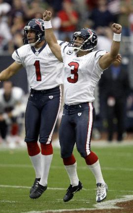
Rob Bironas celebrates.

It is worth noting that a completion could be productive without satisfying the stated productivity criteria. Late in the 4th quarter, December 3 2006, the ball sat on the Colt's 46-yard line. First and 15, Titans’ center Kevin Mawae hiked the ball to Vince Young. Young dropped back and completed a pass over the middle to Travis Henry for an unproductive 4 yards. The Titans shuffled to the line and Young spiked the ball with 15 seconds remaining. Young tossed an incomplete pass on the following play from scrimmage. Fourth and 11, enter Titans’ Rob Bironas who kicked a 60-yard field goal, granting the Titans a 20-17  lead and securing a victory.  Bironas kicked 70% from 50+ yards in his career (24 of 34) but was 1 of 4 kicks of 60+ yards; that 60-yard, game-clinching kick was the longest of his career.  To make apposite of my digression, were Young’s pass to Henry deflected—assuming zero yards were gained on any subsequent play(s)—perhaps Bironas would have missed a 64-yard attempt.  

Table 2. Correlations of Approximated Pass Deflection Yards and Pass Deflections with various variables across team defenses, 2010-2014.

¹Let us verify that PD yards influence field position independently of the effect of the yards allowed on unproductive passes. To do so we regress offensive (of the defensive team) average drive start positions onto unproductive yards and obtain residual values. We regress those residual values onto PD yards and find an infinitesimal decrease in the R2 of drive start on PD yards, from .10 to .08 when controlling for quantity of unproductive pass yardage. Let us then regress average drive start onto the quantities of PDs, obtain residuals, and regress those on PD yardage. Our R2 is essentially zero.

How Defensive Backs Impact Starting Position via Interception Yardage, or SPI%

The previous post discussed Possessions Responsible for Ending, Possessions Ended, and, focally, Possession Recovered. To accompany that, I planned a metric tentatively termed Starting Position Impact, or SPI. Exactly as the term indicates, SPI is designed to account for a DB’s impact on his team’s average starting field position on offense via his defense of the passing game, currently via interception return yardage but, in the future, ideally, also via pass deflections.

Because drive data is readily available for professional teams, I compiled a data set for all NFL teams from regular seasons 2010-11 through 2014-15. I gathered data for 713 player-seasons in that time period for players who, in a given season, suited up for at least four games and netted at least 1 interception. Players who played for multiple teams within a given season were assigned League average Offensive Drive and Average Drive Starting Position values for that season.

IYPOD is Interception Yards Per Offensive Drives. ADSP is Average Drive Starting Position (on offense).

SPI is calculated simply with the above sequence of equations. Table 1 contains the necessary data for the top-35 DBs in SPI since 2010. The top-35, incidentally, are the DBs who are estimated to have increased their teams’ Starting Position by 2% or greater. That is, without these DBs yardage contributions on INT returns, their teams would have started drives that percentage nearer to their own endzone. 

For perspective, I also included in Table 1 Ed Reed (2004) and Darren Sharper (2009) for reference, the top-2 historically in single season INT yards. Likewise, I included IYPOD estimates for seasons from Deion Sanders, Charlie McNeil, and Night Train Lane. For those three, Team Drives were estimated by summing TDs, FGAs, Punts, game kickoffs, and Offensive TOs, and, for Sanders, failed 4^th-down conversion attempts as well.

However, as the regular reader has probably come to realize…I sought a more nuanced and explicatory metric supplementary to SPI. Before I explicate that nuanced metric, however, I will devote the next post to examining how team play on defense and special teams impacts starting field position on offense.

Table 1. Defensive Backs who Increased Their Team's Average Starting Field Position by >2% via INT Yards

Rank	PLAYER	Tm	Year	INT Yds	Drives	Drive Start	Yds/Drives	SPI%
1	Stevie Brown	NYG	2012	307	176	31.4	1.74	5.56
2	Chris Houston	DET	2011	225	197	28.7	1.14	3.98
3	Brandon Browner	SEA	2011	220	192	33.5	1.15	3.42
4	Janoris Jenkins	STL	2012	150	182	24.4	0.82	3.38
5	Ed Reed	BAL	2010	183	189	29.8	0.97	3.25
6	Harrison Smith	MIN	2014	150	176	27.3	0.85	3.12
7	Kerry Rhodes	ARI	2010	174	190	29.7	0.92	3.08
8	Tashaun Gipson	CLE	2014	158	193	26.8	0.82	3.05
9	Rashad Johnson	ARI	2014	146	181	26.9	0.81	3.00
10	Darrelle Revis	NYJ	2011	184	203	30.9	0.91	2.93
11	Ronde Barber	TAM	2012	160	193	29.0	0.83	2.86
12	Tashaun Gipson	CLE	2013	143	195	26.4	0.73	2.78
13	Charlie Peprah	GNB	2011	147	180	30.8	0.82	2.65
14	Chris Harris Jr	DEN	2012	144	188	29.1	0.77	2.63
15	Eric Reid	SFO	2014	138	175	30.5	0.79	2.59
16	Captain Munnerlyn	CAR	2012	107	163	25.5	0.66	2.57
17	Kendrick Lewis	KAN	2011	119	189	24.6	0.63	2.56
18	William Gay	PIT	2014	113	174	25.7	0.65	2.53
19	Matt Giordano	OAK	2011	130	193	27.2	0.67	2.48
20	Brandon Carr	DAL	2012	120	180	27.2	0.67	2.45
21	Brandon Boykin	PHI	2013	136	201	27.9	0.68	2.43
22	Janoris Jenkins	STL	2014	124	186	28.0	0.67	2.38
23	Casey Hayward	GNB	2014	113	169	28.5	0.67	2.35
24	Darius Butler	IND	2012	101	180	24.8	0.56	2.26
25	A.J. Bouye	HOU	2014	120	194	27.7	0.62	2.23
26	Glover Quin	DET	2014	117	179	29.9	0.65	2.19
27	Asante Samuel	ATL	2012	110	175	29.0	0.63	2.17
28	Patrick Robinson	NOR	2012	99	190	24.2	0.52	2.15
29	Tim Jennings	CHI	2013	111	182	28.5	0.61	2.14
30	William Moore	ATL	2010	117	178	31.1	0.66	2.11
31	Richard Sherman	SEA	2013	125	188	31.6	0.66	2.10
32	Malcolm Jenkins	NOR	2010	105	174	29.2	0.60	2.07
33	Devin McCourty	NWE	2010	110	166	32.1	0.66	2.06
34	Brandon Flowers	KAN	2011	95	189	24.6	0.50	2.04
35	Eric Berry	KAN	2013	134	197	33.4	0.68	2.04
	Ed Reed	BAL	2004	358	192	34.2	1.86	5.45
	Darren Sharper	NOR	2009	376	185	31.4	2.03	6.47
	Deion Sanders	SFO	1994	303	198	-	1.53	-
	Charlie McNiel	SDG	1961	349	177	-	1.97	-
	Night Train Lane	LAR	1952	298	171	-	1.74	-

Possessions Recovered by Defensive Backs for his or her Team

Upon completing the last post, I began to wonder: What does INT% really tell us? Indeed, it serves as a statistical alternative to basic percentage of opponents’ passes a player intercepted. INT% attempts to account for the rate at which a player intercepts passes targeted for his assignment. But the actual data are increasingly available, if for a petty membership fee. So perhaps INT% would be useful for historical analyses. I am interested in statistically evaluating defensive backs in the present, however.

Once I completed the INT% analysis and write-up, I considered a statistic to rate defensive backs’ overall impact on opponents’ passing games, as a alluded to at the close of the last post. Ambitiously, I compiled official NCAA statistics for teams and players from 2004, the first year in which pass deflections were officially tracked, through 2014.¹ By the time I compiled all the necessary data and organized it, I had other ideas.

“What does an interception represent for a player and his team?”, I wondered to myself sitting in a theatre watching Pixels. Interceptions represent the gain of possessions for a player's team and the loss of possessions for opponents. That led me to this notion of a statistic to represent the proportion of possessions a DB recovered for his team via his impact on the passing game (i.e., via interception). Or, in other words, the volume of opponents’ possessions a DB ended.

Because team opponent possessions statistics were less than accessible for me, I simply tabulated estimates. To do so I summed each of all TDs scored, FGs, turnovers, punts attempted, and safeties for team offenses 2004 to ‘14, plus the quantity of games (to account for opening or halftime kickoffs). I would have included team attempted FGs but those were unavailable to me and also, blocked kicks but I got lazy. (Fortunately, for NFL stats, team opponent drive statistics appear readily accessible.)

Jayron Hosley defends a pass.

Now, I could have simply divided a DB’s interceptions by opponents’ possessions. But I sought a stat with greater nuance than a simple proportion. So first, in the denominator I divided opponent possessions by 11, the quantity of defensive players on the field. We’ll call that (Opp. Poss. / 11) possessions responsible for ending, or PRE. PRE operates on the premise that each defender is equally culpable for ending opponents’ possessions. However, r = 1 when Possessions Ended is correlated with the basic proportion, INT / Opp. Poss. 

At onset, I anticipated wanting to somehow weight the values in the numerator and denominator to reward the DB whose offensive teammates were counterproductive. For instance, in 2010 Jayron Hosley of Virginia Tech intercepted 9 passes. In 2006, John Talley of Duke intercepted 7 passes. For the seasons in reference, Hosley’s ended 5.4% of opponents’ possessions and Talley, 5%, proportionately. The Possessions Ended formula puts Hosley at .59 (8th highest) and Talley at .55 (tied for 12th highest).  

In 2010, VT finished 11-3 and 8-0 in ACC play whereas in 2006, Duke finished 3-9 and 1-7 in ACC play. Hosley’s 2010 offensive teammates relinquished only 13 turnovers and scored 80 times whereas Talley’s 2006 offensive teammates relinquished 31 turnovers and scored only 28 times. Thus, Hosley’s offensive teammates increased his PRE more so by scoring whereas Talley’s offensive teammates increased his PRE more so by fumbling and throwing interceptions.

So I settled on the Possessions Recovered formula above. I considered weighing Player Int’s by the sum of turnovers and punts but, although both are bound to occur, punting seems to me unproductive rather than counterproductive. With turnovers, Talley’s numerator is larger than Hosley’s because his offensive teammates generated more turnovers. In the denominator, I weighted PRE by scores. Therefore, Talley’s denominator is smaller than Hosley’s because his offensive teammates scored less often. Do note that Team Scores excludes safeties and includes TDs scored on defense and special teams.

Table 1 appears at the bottom of the page and includes the basic proportional possessions ended, the Possessions Ended, and Possessions Recovered, as well as the rankings for the latter two stats. I included in Table 1 players who were top 25 in Possessions Ended and Possessions Recovered to provide the reader some perspective on the nuance of Possessions Recovered. With Possessions Recovered we see that 2006 John Talley has risen to the number-one spot with 61.3% of PRE whereas 2010 Jayron Hosley has plummeted to 320th with 9.6% of PRE. We also find for instance, Chris Prosinski, presently three years into his pro-career, sitting at 14th with 30.3% Possessions Recovered. Prosinski picked off 3 passes in 2008 for a Wyoming team that turned the ball over 36 times and scored only 26 times. Possessions Recovered is also sensitive to interception totals as 2014 Gerod Holliman was at 8th with 34.1% for a Louisville team that committed 26 turnovers and scored 66 times.  

John Talley manufacturing yardage.

There are shortcomings to PE and PR, of course. PE essentially mirrors the proportion of interceptions to opponents possessions, as discussed above. PR is of course more sensitive to DBs who play for programs with counterproductive offenses. Surely other weaknesses could be identified. To improve either PE or PR, the quantity of passes deflected or broken up by a DB could be divided by three or four and that quotient summed with total interceptions in the numerators. Doing so is based on the premise that three or four downs ended by a deflected pass would equate to a possession. I would opt for four for parsimony. 

Let us return to the players discussed in my example above. Jayron Hosley was drafted in the third round of the 2012 draft by the New York football Giants. Some would describe his professional performance as "unsatisfactory." But what about John Talley? 

John Talley is one of 4 players for whom I had three years of data. His junior and seniors seasons rank in the top-10 of Possessions Recovered. But what became of Mr. Talley? Talley was rated 33 of 218 cornerbacks available in the 2007 NFL draft. Fellow 2007 DB prospects Leon Hall, Darrelle Revis, et al. are currently active on NFL rosters but like Al Worley before him, Talley passed undrafted (Worley: 172.3% of PRE for a 3-5-2 UW team with 38 TOs and 23 scores).

Talley’s pro-day weight of 171lbs is 20lbs under the average of the top-30 projected CBs in the 2007 NFL Draft. Perhaps a pro-day 40yd-dash of 4.61s resulted in Tally’s exclusion from the NFL Combine. None of first-30 CBs had 40yd-dash times slower than 4.56. The top-30 averaged about 15 reps on the 225lb-bench press; the lowest quantity, 10. Talley did 9. His 9’11” broad jump was slightly below average of 10’1” and a 32’6” vertical jump was below the average of 35’3”.

Talley’s 3-cone drill time of 6.77s was faster than the average of 6.96s and faster than 75% of the top-30. Considering 60 CBs drafted since 2005, Talley’s 6.77s on the 3-cone drill is in the 72nd percentile. Considering 170 WRs drafted since 2000, Talley’s 6.77 is in the 78th percentile, suggesting Talley may have possessed the agility necessary to compensate for the cutting and curling routes run by NFL receivers, many of whom would outsize, outleap, and outsprint him.

Talley deflects a pass targeted for Young Megatron.

In 2005 and 2006, John Talley was given the arduous task of guarding Georgia Tech phenomenon Calvin Johnson. Now better known as Megatron, the 6’5” Johnson and his 4.35s 40yd-dash were a mismatch for Talley. But Talley held his own in two Duke losses against GT. Johnson caught 4 passes in ’05 and 5 in ’06 for 73 and 78 yards, respectively. 

Talley held Johnson without a TD catch in ’05 while deflecting 1 pass and intercepting another. In ’06 however Johnson grabbed 2 TD catches only playing in the first half—due, at least partially, to a counterproductive offense that failed to keep Duke in the game. Of Talley’s 2 deflections of passes targeted for Johnson in ’06, one led to an interception.  

I briefly reviewed the box scores for the 2005 and '06 games, and by my estimation Johnson was targeted 8 and 7 times, respectively. If the box scores read accurately, then Talley actively defended (i.e., INT or deflection) 25% of passes targeted for Johnson in 2005 and 28.9% in '06.

Aside from Johnson’s TD production, his stat lines are nearly identical in the two games. Johnson suggested that he was triple-teamed in ’05; Talley contended otherwise but acknowledged that Johnson did demand “extra attention.” Likewise, Talley’s defensive production was similar in both games. Of Johnson’s 2 career tackles, 1 was of Talley in ’05. Summarily, in two showdowns with Talley, Johnson's production was tantamount to his collegiate averages. 

We know what Megatron became and what he continues to become. But as for Talley, his Twitter profile indicates that he is now a father. Since completing his BA in African American Studies at Duke in 2007, Talley earned his MBA back in 2012. From what I can gather, he currently teaches sixth grade mathematics.² In my opinion, following 18 years of education, Mr. Talley offers fair test-correction and tutoring policies to his students. Likewise, his expectations of classroom behavior are reasonable. Let us hope that as an educator, Mr. Talley’s pupils fare better with him than Calvin Johnson did—that is, let us hope Talley's pupils fare better than average.

Table 1. Top-25 NCAA DBs from 2004-2014 in Possessions Ended or Possessions Recovered³

Player	Year	Program	PE Rank	PR Rank	G	INT	Opp. Poss.	Team TOs	Team Scores	Basic %	PE	PR
John Talley	2006	Duke	12	1	12	7	139	31	28	0.05	0.55	0.61
Lionell Singleton	2006	Florida Int'l	109	2	10	5	142	26	20	0.04	0.39	0.50
Stanley Franks	2006	Idaho	3	3	12	9	145	26	36	0.06	0.68	0.49
Domonic Cook	2010	Buffalo	75	4	12	6	155	33	29	0.04	0.43	0.48
Anthony Smith	2005	Syracuse	68	5	11	6	152	27	27	0.04	0.43	0.43
David Amerson	2011	NC State	2	6	13	13	166	25	59	0.08	0.86	0.37
John Talley	2005	Duke	109	7	11	5	142	26	29	0.04	0.39	0.35
Brian Lainhart	2009	Kent St.	32	8	12	7	156	28	40	0.04	0.49	0.35
Gerod Holliman	2014	Louisville	1	9	13	14	178	26	66	0.08	0.87	0.34
Anthony Harris	2013	Virginia	18	10	12	8	167	26	42	0.05	0.53	0.33
Trae Williams	2006	South Fla.	22	11	13	7	149	29	47	0.05	0.52	0.32
Jack Williams	2005	Kent St.	248	12	11	4	146	31	30	0.03	0.30	0.31
Khayyam Burns	2006	Arkansas St.	181	13	12	4	129	30	33	0.03	0.34	0.31
Chris Prosinski	2008	Wyoming	430	14	12	3	151	36	26	0.02	0.22	0.30
Anwar Phillips	2004	Penn St.	191	15	11	4	132	27	31	0.03	0.33	0.29
Morgan Burnett	2008	GT	12	16	13	7	139	27	52	0.05	0.55	0.29
Senquez Golson	2014	Ole Miss	4	17	13	10	165	25	58	0.06	0.67	0.29
Sean Baker	2010	Ball St.	75	18	12	6	155	31	46	0.04	0.43	0.29
Rahim Moore	2009	UCLA	4	19	13	10	165	24	56	0.06	0.67	0.29
Eric Berry	2008	UT	10	20	12	7	135	18	36	0.05	0.57	0.29
Julius Stinson	2007	Wyoming	146	21	12	5	153	31	41	0.03	0.36	0.27
Dion Byrum	2005	Ohio	60	22	11	6	146	18	30	0.04	0.45	0.27
Reggie Corner	2007	Akron	37	23	12	7	158	25	45	0.04	0.49	0.27
Chaz Williams	2005	ULM	87	24	10	5	134	25	38	0.04	0.41	0.27
Charles Gordon	2004	Kansas	25	25	11	7	152	23	44	0.05	0.51	0.26
Dwight Lowery	2006	SJ St.	6	26	13	9	151	21	52	0.06	0.66	0.26
Kevin Sanders	2008	UAB	16	27	12	7	146	25	50	0.05	0.53	0.26
Quinten Rollins	2014	Miami (OH)	14	35	12	7	142	20	44	0.05	0.54	0.25
Quintin Demps	2006	UTEP	19	43	12	7	147	25	57	0.05	0.52	0.23
Ryan Smith	2006	UF	11	54	14	8	157	24	63	0.05	0.56	0.21
Daymeion Hughes	2006	Cal	9	87	13	8	153	22	69	0.05	0.58	0.18
DeAngelo Smith	2007	Cinci'	24	93	13	8	173	26	74	0.05	0.51	0.18
Larry Parker	2011	SD St.	22	164	13	7	149	16	59	0.05	0.52	0.14
Manti Te'o	2012	Notre Dame	15	186	13	7	143	15	62	0.05	0.54	0.13
Darcel McBath	2008	Texas Tech	19	203	13	7	147	21	86	0.05	0.52	0.13
Joe Pawelek	2008	Baylor	19	270	12	6	126	11	52	0.05	0.52	0.11
Robert Lester	2010	'Bama	7	274	13	8	145	14	77	0.06	0.61	0.11
Jayron Hosley	2010	VT	8	328	13	9	168	13	80	0.05	0.59	0.10
Anthony Wright	2009	Air Force	16	336	13	7	146	12	68	0.05	0.53	0.09
Al Worley	1968	Washington			10	14	136	35	23	0.10	1.13	1.72

Notes:

¹ All data were obtained directly from the Division 1 Statistics listed on NCAA.org; spreadsheets available upon request.

² Although I do attempt to provide the reader novel content, I refuse to make this an expose on a man's private life. But with some digital digging I was able to find this indicating Mr. Talley's status of educator. I have made an attempt to conceal identifiers of Mr. Talley's whereabouts and contact information in respect to his rights to privacy.

³ Shown at bottom is PE and PR for Al Worley. Team data for Al Worley were obtained from UW media guide here.

eINT%, or DB Interceptions Per Passes Targeted for his or her Coverage Assignment

The first gal I crushed on as a youth was a brunette named Kelly. Aside from chasing each other to a clearing in the woods, basketball was the first sport I loved. The Michael Jordan concept was my favorite. I watched Come Fly with Me on repeat. I probably watched NBA Jam Session more frequently, though, and religiously read the compendium text still nestled on my bookshelf today.

However, Jordan departed from the game in 1993. Likewise, the fam’ and I were relocated southward by my father’s acquisition of stable employment. Aside from teenage pregnancy, obesity, substandard education, joblessness, voting against self-interests, poverty, and libidinous religiosity, the biggest thing in the South is college football. In New England the professional gridiron game received greater coverage than the collegiate game that ruled in my new stomping ground.

At 8, I was oblivious to the nuances of the two and probably watched pro-games because it was more familiar. Today I prefer the myriad offensive stratagems seen in the college game to the “retreaded” schemes of the pros.  But really, it is college football and nothing is comparable.

1996 Deion Sanders Air Max Diamond Turf.

To the 8-year old Justin, the New England Patriots were unappealing. The 49ers had won 4 titles in the 1980s and my grandparents lived in the greater San Fran area. So I cheered for the 49ers. Deion Sanders joined the San Francisco 49ers for the 1994 season and Prime Time became my favorite player, easy. He shut down opposing receivers. He scored touch downs on defense as he high-stepped into the endzone. Two years later, when I entered middle school and appearances suddenly mattered, I begged and begged my parents for Air Max DTs seen at right. 

Importantly, all the kids I knew from school and from the after school program I attended, all those kids’ favorite players were quarterbacks, running backs, and wide receivers. Being the new kid, I found some comfort because my intentions to play cornerback were rarely contended when we played a slightly more bellicose variety of two-hand touch. 

I played baseball, basketball, and soccer through my early adolescence. However, my mother prohibited playing football until I was a teenager. Ultimately, much of my adolescence was devoted to strumming guitars and staring into the sun but needless to say, she probably would have forbidden my donning shoulder pads then too. Had I tried out though, it would have been for spot in the defensive backfield.

Salient for aspiring defensive backs is the number 14. Coincidentally, 14 interceptions is the single season record in both the professional and collegiate ranks, achieved long-ago by ‘Night Train’ Lane (1952, LA Rams) and Al Worley (1968, UWash), respectively.

Night Train hawks the ball.

Ella Lane recovered the 3-month old Lane from a dumpster, adopted him into her family, and reared the future game-changer.  Night Train later served 4 years as a Lt Col in the US Armed Services during the Second World and Korean Wars. After discharge, Lane walked on as a third string receiver and was repurposed as a defensive back prior to his rookie season. That was the same season in which he snagged the 14 INTs. Some speculate that Lane originated the cornerback blitz as QBs increasingly avoided targeting the receivers he covered. 

Lane was married to the renowned Dinah Washington before her death. After football, Night Train was inducted into the Hall of Fame and coached for various small college programs.  Dick Lane, as he was known to friends and family, was survived by three sons and several grandchildren when he passed in 2002 from ailments indicative of a football life.

Elven 'Al' Worley

Less is available about Elven ‘Al’ Worley. He was a consensus All-American in his final season as a Washington Husky in 1968, the season in which he nabbed 14 passes thrown by opposing QBs. During his time at UW Al was a member of the ROTC. Worley was touted among the top DBs in the 1969 draft yet he is missing from the 71 defensive backs selected in the 1969 NFL draft.¹ At 5’11” 175lbs, Worley was admittedly slow and slightly underweight compared to 223 defensive backs whose rookie seasons fell in the seasons 1965-70.  Perhaps these factors limited his potential in the eyes of NFL scouts. Worley did play in 1969 a year of pro football for the since-defunct Continental Football League, however. As an All-Pro All-Star defensive back for the Seattle Rangers he intercepted 4 passes.
 
Ostensibly, Worley later completed his bachelor’s degree at UW in 1970 while serving as an assistant coach to the football team. Worley was appointed defensive backs coach at Northern Arizona in 1971 and held the position through at least 1974.  By 2003 Al Worley resided in Hawaii.²  Maybe he still does. He might live in Huntington VA, though, or perhaps he holds a membership to a Texas RV club. Who knows, I'm no private investigator nor is this an expose of one man's private life. In June 2015 Al Worley was included on the 2016 College Football Hall of Fame ballot. 

Lester Hayes' unique pre-snap stance.

One of Holliman's interceptions of Jameis Winston in 2014.

No pro pigskin player has approached Lane’s mark since Lester Hayes did in 1980 with 13.  Prior to 2014, two had flirted with Worley’s record, David Amerson (2011, NC State) and Terrell Buckley (1992, FSU), who each snagged 13. Enter Gerod Holliman, former free safety of the Cardinals who represent Louisville, capital of Louisville. By early November 2014, I noticed Holliman’s total was 10 and then, a game later, 13. Ultimately, Holliman tied Worley’s record.  

Having known Worley’s fate of undrafted peril, I wondered how Holliman would fare in the 2015 draft. That led to my curiosity about an objective valuation of a DB’s ability to intercept passess. Specifically, the consistency and reliability with which a DB generates interceptions when the pass is targeted to his assignment(s). For instance, in 2003 Josh Bullocks snared 10 INTs for Nebraska, getting at least 1 INT in 9 of 11 games.  Compare that to 2009 UCLA's Rahim Moore who totaled 10 INT in 2009 but only 1 INT in 6 of 13 games. Moore intercepted multiple passes in multiple games but Bullocks appears more likely to have intercepted a pass in any given game. Notably, although Moore played in a greater quantity of games, Bullocks’ opponents attempted 430 passes where as Moore’s opponents attempted only 367.

I advise the reader, my acumen for mathematics is comparable to neither Brian Burke nor Gerald Tamayo. Uncertain how to begin I referred to a familiar statistic, the shot-block percentage (BLK%) used in basketball. BLK% is intended to provide an estimation of the percentage of opponents' 2-point shots a player blocked while he or she was playing. I contemplated several configurations for INT% formulas. However, BLK% translates inexactly to INT% because a constituent of BLK% is a players' minutes played. Minutes played is a readily accessible basketball statistic but in football statistics, the quantity of plays in which a player plays is generally inaccessible. 

Ok, so with that stated I based the final formula on several premises. First, there are a maximum of five eligible receivers on any given play. Second, thorough analysis by others indicates that ~68% of passes are targeted to eligible receivers lined up out wide or at the slot. To obtain that percentage, I included WRs out-wide or at slot, RBs out-wide or at slot, and TEs out-wide. TEs lining up at the slot were excluded because, due to their physical statures, my thinking is that they were generally covered by an LB. 

Thus, there are two probabilities to consider. The first is the probability that an eligible receiver will be targeted (i.e., 1/5). The second is the probability that a pass is targeted for an eligible receiver that would be covered by a DB (i.e., .68). I like this notion of probability because, if the DB of interest is a second-stringer, we could perhaps adjust the first probably to 1/10. Likewise, the second probability could be adjusted for LBs or DLineman (perhaps, .32). 

So in the numerator is the quantity of interceptions by a DB. In the denominator is the quantity of pass attempts defended by that DB's team multiplied by the first probability, .20 or 1/5. The product thereof is multiplied by .68, the second probability. Although the probabilities used in the INT% formula are the most rudimentary of estimates, the results are interesting. 

Table 1. Estimated-INT% for Selection of NCAA DBs with >= 10 INTs in a Season

Player	Year	Program	G	INT	Pass	%Pass Int	eINT%
Al Worley	1968	Washington	10	14	203	6.9	50.7
Gerod Holliman	2014	Louisville	13	14	410	3.4	25.1
Dre Bly	1996	UNC	11	11	326	3.4	24.8
Terrel Buckley	1992	FSU	13	13	402	3.2	23.8
David Amerson	2011	NC State	13	13	407	3.2	23.5
Sean Taylor	2003	Miami	13	10	328	3.0	22.4
Dwight Smith	2000	Akron	11	10	337	3.0	21.8
Rahim Moore	2009	UCLA	13	10	367	2.7	20.0
Anthony Floyd	2000	Louisville	11	10	389	2.6	18.9
Jim Leonard	2002	Wisconsin	14	11	432	2.5	18.7
Senquez Golson	2014	Ole Miss	13	10	402	2.5	18.3
Aaron Beasley	1994	WVU	12	10	402	2.5	18.3
Josh Bullocks	2003	Nebraska	13	10	430	2.3	17.1

Table 1 provides INT% and the necessary data for Worley and players who tallied 10 or more INTs in the past quarter century, sorted descendingly by INT%.³ Worely's feat is given some perspective. The second-to-rightmost column of Table 1 displays the basic percentage of opponent passes intercepted. Unfortunately for my inchoate INT%, the table demonstrates that INT% provides little additional nuance beyond the basic percentage. That is, the rankings of INT% essentially mirror that of basic percentage. However, we gain insight into my earlier discussion of Rahim Moore and Josh Bullocks. INT% suggests that Moore was somewhat more adept at intercepting passes than Bullocks, a result probably attributable, at least mathematically, to Moore's team defensing fewer passes. But again, Moore's basic percentage was slightly greater than that of Bullocks.

The lack of nuance aside, ideally, INT% provides us an estimation of the rate at which a defensive back intercepts passes thrown to the receiver he was defending. But is the INT% ecologically valid? That is, if we knew the actual quantity of passes available for a player to intercept, would INT% provide an accurate estimate?

Table 2. Actual- and Estimated-INT% for a Selection of 2014 NFL DBs

Player	Team	Targeted	INT	PASS	INT%actual	INT%estimate	Act - Est
Richard Sherman	SEA	65	4	507	6.15	5.80	-0.35
Darrelle Revis	NE	79	2	574	2.53	2.56	0.03
Casey Hayward	GB	26	3	564	11.53	7.82	-3.72
Rashean Mathis	DET	89	1	592	1.12	1.24	0.12
Antonio Cromartie	ARZ	81	3	579	3.72	3.81	0.11
Chris Harris	DEN	89	3	641	3.37	3.44	0.07
Josh Wilson	ATL	37	1	566	2.70	2.60	-0.10
Brice McCain	PIT	51	3	543	5.88	4.06	-1.82
William Gay	PIT	104	3	543	2.88	4.06	1.18
A.J. Bouye	HST	85	3	619	3.53	3.56	0.03
Bradley Fletcher	PHI	115	1	591	0.87	1.25	0.37
Blidi Wreh-Wilson	TEN	76	1	545	1.32	1.35	0.03
Joe Haden	CLV	113	3	587	2.65	3.76	1.10
Kyle Fuller	CHI	101	4	548	3.96	5.37	1.41
Buster Skrine	CLV	123	4	587	3.25	5.01	1.76
Jason McCourty	TEN	125	3	545	2.40	4.05	1.65
Johnathan Joseph	HST	117	2	619	1.71	2.38	0.67
				Mean:	3.50	3.65	0.15
				SD:	2.53	1.74	1.32
Note, italicized eINT%s were computed with .1 in denominator instead of .2 because those players were considered second-string following cursory comparison of their quantity of games started and games played.

Let us consider 17 professional defensive backs for whom we the have numbers. Table 2 contains the actual INT%, our estimated INT%, and the difference of the two. For these 17 players, the eINT% formula overestimates the actual INT% by an average of .15 and, if we exclude an outlier of -3.72, an overestimation of .39. (Actual and estimated INT% correlated positively, Rho = .85, p < .001, 2-tailed.)⁴

There are shortcomings to predicted INT%, of course. The pro-sample used to validate the accuracy of the eINT% is small. The accuracy of eINT% may be less evident with a larger data set. But given my fixed income as a grad student, I am unwilling to spend the money to obtain targeted-data for the League. 

For the college and professional samples, estimated INT% increases as opponents' pass attempts decrease; the college sample considerably more so than the pro sample (act. Rho = -.35, est. r = -.35, ps > .15), skewed by the Worley data point (Rho = -.46 with Worley, Rho = -.32 without, ps > .10). Also, each team in the college sample defended more run than pass plays whereas more pass than run plays were defended in the pro sample. 

Probabilistically allocating opponents' pass attempts equally among defensive backs led, at least in part, to disparities that emerged between actual- and estimated-INT% in the pro sample. Inclusion of another readily accessible statistic of individual players might provide a more accurate and personalized estimate of INT%. This is evident in the pro-sample as Brice McCain and William Gay each tallied three interceptions for the Pittsburgh Steelers and thus have identical estimated INT% despite Gay being targeted more than twice as often as McCain.

I am fond of the relative simplicity of the statistic, however. The formula could be easily enhanced by summing interceptions and pass deflections to provide a statistic more representative of a DB's ability to prevent successful passing.

Before concluding, let us return to Al Worley and 1968. Football strategies have shifted and that is evident in the statistics. The ratio of pass to run plays has increased. Rules have changed. Fewer passes were attempted in '68 and Worley's 50.7 estimated INT% is gaudy, indeed. Recall, the highest actual-INT% in the pro-sample was Casey Heyward's 11.43 and, in estimated-INT%, Howard's 7.82; his basic INT percentage was 0.5% (excluded from Table 2 due to minuteness). Consider then, Night Train Lane's basic percentage of 3.9% in his record breaking 1952 season and an estimated 28.6 INT%. Staggering. Lester Hayes picked off 2.5% of opponents' passes in 1980 with an estimated 18.2 INT%. My favorite, Prime Time, well, in his best season, he picked 1.4% on 7 interceptions in 1993 with an eINT% of 10.2 and in the '94 season with the 49ers, he had 6 picks at 1% with an eINT% of 7.6.

So I leave the reader with INT%, for now. To follow in the near future are my thoughts on statistically evaluating a defensive back's ability to counteract his opponents' successes scoring and moving the ball. 



Notes:

¹ As an aside, Roger Wehrli played was a 7-time All-Star in his 14-year NFL career.  

² Admittedly, I'm wagering that the obituary is of a woman who is Worley's sister. The 1968 Walla Walla Union-Bulletin snippet indicates Worley is one of 10 children and the 2003 obituary states the woman was survived by 5 brothers and 4 sisters. The WWUB snippet mentions Al's brother Larry and the obituary mentions a brother named Lawrence which is often short for Larry. However, the WWUB snippet states the mother's name is Blanche whereas the obituary states the mother's name is Bertha. Regardless, I am writing this text to discuss estimated INT% absent any intentions of unearthing a man's private life. However, the reader curious about Worley's later life may find this worth noting.

³ Unless noted, all statistics sourced from Sports-Reference.com. Less accessible sources are provided for the reader's convenience.

⁴ Here and elsewhere in the text, Rho, or Spearman's rank correlation, is presented when data have high skewness and/or kurtosis.